Not All Network Traffic Is Equal
In a conventional enterprise environment, a single network fabric handles everything: user traffic, application data, storage I/O, management communications, and backups. For general-purpose workloads, this approach is adequate. The traffic volumes are modest, the latency requirements are loose, and occasional contention is tolerable.
AI workloads break this model. A multi-GPU training job generates two fundamentally different types of network traffic simultaneously, and each type has distinct requirements. When both traffic types share the same physical network, they interfere with each other in ways that degrade the performance of both. Understanding this interference—and designing networks that prevent it—is one of the most impactful decisions in AI infrastructure planning.
Compute Fabric vs Storage Backbone
The two traffic categories in an AI workload are the compute fabric and the storage backbone, and they behave very differently.
Compute Fabric Traffic
During distributed training, GPUs across multiple nodes must exchange gradient updates after each training step. This communication pattern is characterised by frequent, relatively small messages that must arrive with minimal delay. The collective operations involved—all-reduce, all-gather, broadcast—are synchronisation barriers: every GPU waits until all GPUs have finished communicating before the next training step can begin. A single slow link delays the entire cluster.
For this traffic, latency is the dominant concern. The total data volume per exchange may be modest (megabytes to low gigabytes), but the frequency is high and the tolerance for delay is near zero. Technologies like InfiniBand and RDMA (Remote Direct Memory Access) exist specifically to serve this pattern, bypassing the operating system's network stack to deliver single-digit microsecond latencies.
Storage Backbone Traffic
Simultaneously, each GPU node is reading training data from storage. This traffic pattern is the inverse of compute fabric traffic: it involves large, sustained data transfers—streaming gigabytes of images, sequences, or numerical arrays—where bandwidth is the dominant concern. A few extra microseconds of latency per request are tolerable, but throughput that drops below the rate at which GPUs consume data causes idle time.
Storage traffic is also inherently bursty. Data loaders prefetch batches, creating periodic spikes in network utilisation. When these spikes collide with compute fabric traffic on a shared network, both suffer: gradient exchanges are delayed by storage bursts, and storage throughput is throttled by quality-of-service policies protecting compute traffic.
Mixing compute and storage traffic on a single network is like running a courier service and a freight operation on the same single-lane road. The couriers need speed; the trucks need capacity. Neither gets what it needs.
When Bandwidth Matters vs When Latency Matters
A common mistake in network design for AI is treating bandwidth as the universal metric. Organisations see that 100 GbE offers ten times the bandwidth of 10 GbE and assume that deploying 100 GbE everywhere solves all problems. It does not, because bandwidth and latency address different bottlenecks.
Bandwidth matters when the workload involves moving large volumes of data continuously. Storage reads during training, checkpoint writes, and dataset transfers between tiers are all bandwidth-sensitive. For these operations, 100 GbE (or faster) provides the sustained throughput needed to keep GPU data pipelines full.
Latency matters when the workload involves frequent synchronisation between distributed processes. Gradient exchanges in data-parallel training, parameter updates in model-parallel training, and metadata lookups on distributed filesystems are all latency-sensitive. For these operations, the absolute bandwidth may be less important than the time it takes for a single message to traverse the network.
This is why 10 GbE and 100 GbE coexist in well-designed AI infrastructure. A 10 GbE network may be entirely adequate for management traffic, monitoring data, and low-bandwidth services, while 100 GbE (or InfiniBand) is reserved for the traffic that actually affects workload performance. Deploying the same speed everywhere wastes budget on links that do not need it and, worse, provides a false sense of uniformity that obscures the real performance constraints.
Segmentation, Isolation, and Performance Predictability
Physical network separation—using distinct switches, cables, and interfaces for compute and storage traffic—provides the strongest isolation. Each fabric operates independently, and contention on one cannot affect the other. This is the gold standard for production AI environments.
Where physical separation is not feasible, logical segmentation through VLANs and quality-of-service (QoS) policies can provide a degree of isolation. However, logical segmentation has limitations. QoS policies manage contention; they do not eliminate it. Under sustained high load, a shared physical fabric will still experience interference between traffic classes, even with well-configured QoS. The result is performance variability—exactly the condition that makes AI workload scheduling unpredictable and validation baselines unreliable.
Key segmentation practices for AI networking include:
- Separate physical networks for GPU interconnect and storage I/O. This is the single most impactful architectural decision for multi-node training performance.
- Dedicated management network. Keep SSH, monitoring, IPMI/BMC, and administrative traffic off the data path entirely. Even small amounts of management traffic can introduce jitter on latency-sensitive fabrics.
- Non-blocking switch topologies. Ensure that the aggregate bandwidth of all connected ports equals or exceeds the switch's backplane capacity. Oversubscribed switches introduce contention at the infrastructure level that no software configuration can resolve.
- Jumbo frames on storage networks. Increasing the maximum transmission unit (MTU) from the default 1,500 bytes to 9,000 bytes reduces per-packet overhead and improves throughput for large sequential transfers. This is a simple change with measurable impact on storage network performance.
A Practical Benchmark Plan Before Committing
Network specifications on data sheets describe theoretical maximums. Real-world performance depends on switch configuration, cable quality, firmware versions, driver settings, and workload characteristics. Before committing to a network architecture, run controlled benchmarks that reflect your actual workload patterns.
- Baseline single-link throughput. Use
iperf3or equivalent to measure raw TCP throughput between two nodes on each network. Compare against the theoretical link speed. You should achieve at least 90 percent of line rate for large transfers. - Multi-stream contention test. Run simultaneous transfers from multiple nodes to a single storage target. Measure how throughput per stream degrades as the number of concurrent streams increases. This reveals switch and storage controller bottlenecks.
- Latency under load. Measure round-trip latency on the compute fabric while simultaneously generating storage traffic. If compute-fabric latency increases by more than 10 to 15 percent when storage traffic is active, isolation is insufficient.
- Realistic workload profiling. Run an actual training job on a small subset of nodes and capture network utilisation, latency distributions, and GPU utilisation simultaneously. Correlate periods of low GPU utilisation with network events to identify bottlenecks.
- Failure scenario testing. Disable a link or switch port and verify that failover works correctly and that performance degradation is within acceptable bounds. Document the failover time and steady-state performance with reduced redundancy.
These benchmarks should be completed before production workloads are deployed, and the results should be retained as baseline documentation. When performance questions arise later—and they will—having a validated baseline makes diagnosis dramatically faster.
Separate compute and storage networks prevent cross-traffic bottlenecks that silently degrade AI workload performance. This is not optional complexity—it is the architectural foundation that makes GPU utilisation predictable, training schedules reliable, and infrastructure investment defensible.
Network design is invisible when it works and catastrophic when it does not. Investing in proper segmentation and benchmarking before deployment avoids the far more expensive process of diagnosing mysterious performance degradation after your GPUs are already in production.
References & Further Reading
- NVIDIA RTX A6000 Datasheet Product specifications including NVLink combined memory context relevant to "96 GB" VRAM messaging.
- NVIDIA A100 Tensor Core GPU Data centre GPU specifications for high-performance AI training and inference workloads.
- NVM Express Base Specification NVMe protocol specification — explains why NVMe delivers lower latency and better scalability for SSD access than legacy interfaces.
- NVMe Overview High-level overview of NVMe design goals including latency reduction, scalability, and bandwidth/IOPS improvements.
- IETF RFC 7530: NFSv4.0 Protocol Canonical NAS protocol standard — useful reference for shared storage architecture discussions.